How to reclassify variables in Stata
Welcome to the Stata Guide on how to reclassify variables! In this guide, we’ll cover three different ways of reclassifying variables:
- Continuous → Categorical
- Categorical → Categorical
- Categorical → Binary
Before we begin learning the commands to do so, let’s review these different variable types and their various uses and interpretations.
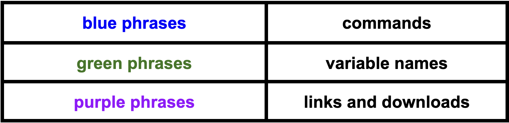
Guide Legend:
Continuous Variables
Continuous variables are a subcategory of numerical (or quantitative) variables which can take on an infinite number of values within a given range. Some examples of common measurements which they can represent include temperature, weight, price, and age. This variable type often takes on fractional and decimal values depending on the specificity of the units being measured. Continuous variables can be placed in contrast with discrete variables. Discrete variables are those which can only take on separate and specific values and which can be counted (i.e. population, class size, or pages in a book).
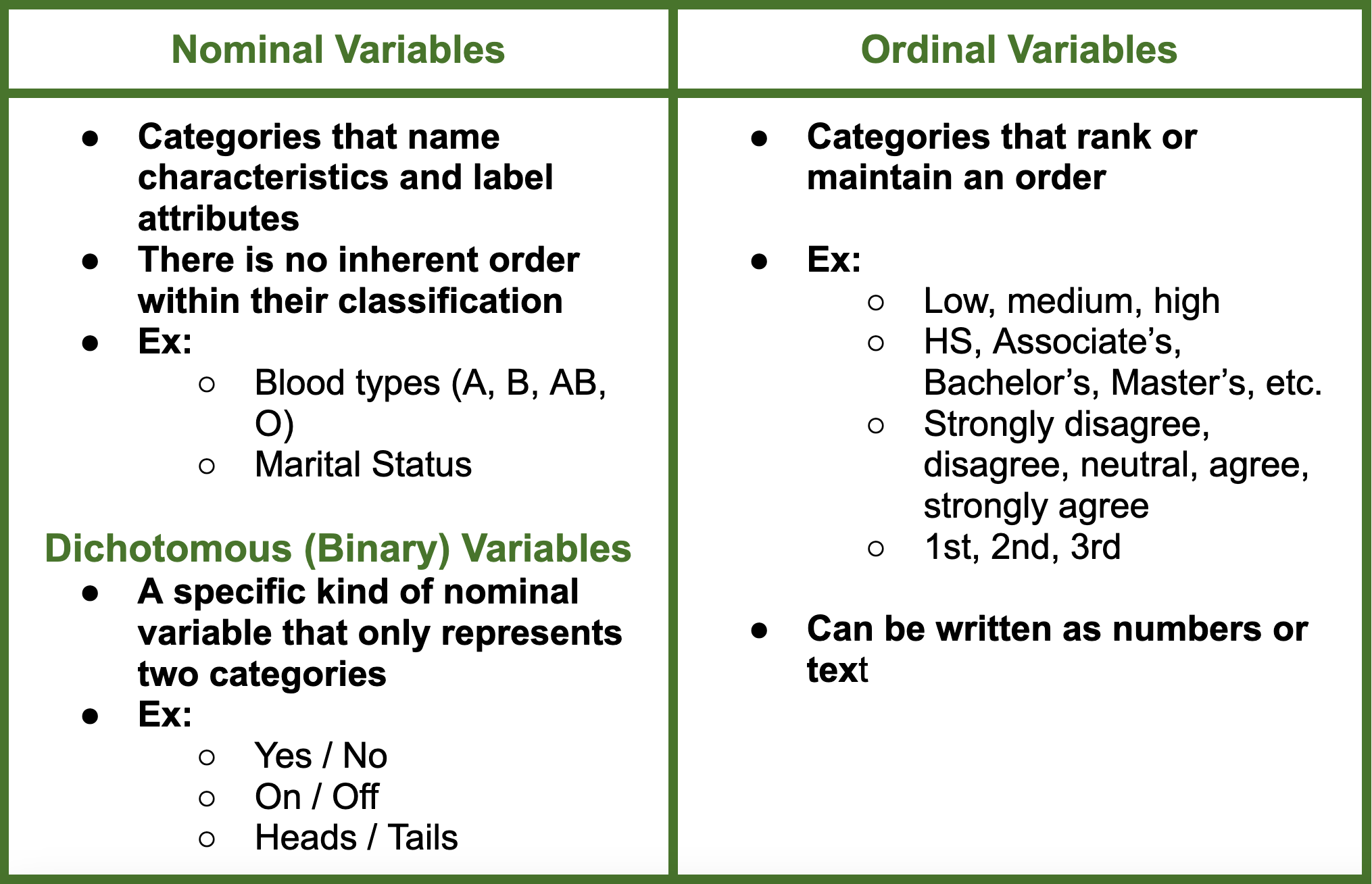
Categorical Variables
Categorical variables are those which take on a fixed number of values and specify observations based on their belonging to a group (or ‘category’). Examples of common categorical variables include income bracket, blood type, education level, and race. Categorical variables can be useful when making cross-group comparisons, especially within policy analysis.
There are three broad categories under which categorical variables can be broken down into:
There are three broad categories under which categorical variables can be broken down into:
When would you want to reclassify a continuous variable as categorical?
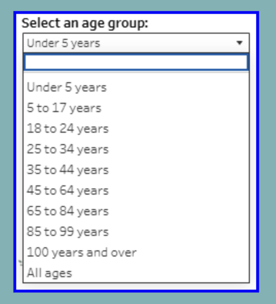
Throughout social research, lumping a variable by category can assist in ease of analysis. The 2020 census’ grouping of age into 9 buckets is a primary example of how a continuous variable can be broken into categories to make stating relationships easier. Within this guide, we will be focused specifically on reclassifying the age variable as categorical.
*See Exploring Age Groups in the 2020 Census.
Similarly, years of education are often seen classified as corresponding to the degrees they represent instead of merely years. This allows for a more accurate understanding of the complex interrelationships between a variety of factors. More simply, when the degree associated with years of schooling can’t be clearly determined (as in our case), years of education can be reclassified as low, medium, or high.
Similarly, years of education are often seen classified as corresponding to the degrees they represent instead of merely years. This allows for a more accurate understanding of the complex interrelationships between a variety of factors. More simply, when the degree associated with years of schooling can’t be clearly determined (as in our case), years of education can be reclassified as low, medium, or high.
I. Reclassifying Continuous Variable as Categorical
We’ll be using a Kaggle KNN dataset to learn the reclassifying process. You can download this data by clicking here. This is a dataset which covers demographic information such as income, age, race, gender, relationship status and more.
Here is the. Do file with all the steps covered within this guide.
Let’s begin by a) opening Stata, b) setting the working directory, c) importing our Kaggle Adult Income dataset, and d) opening a .do File.*
*For an in-depth guide on how to complete this, see the general Stata Guide.
Once this has been completed, your interface should resemble the following:
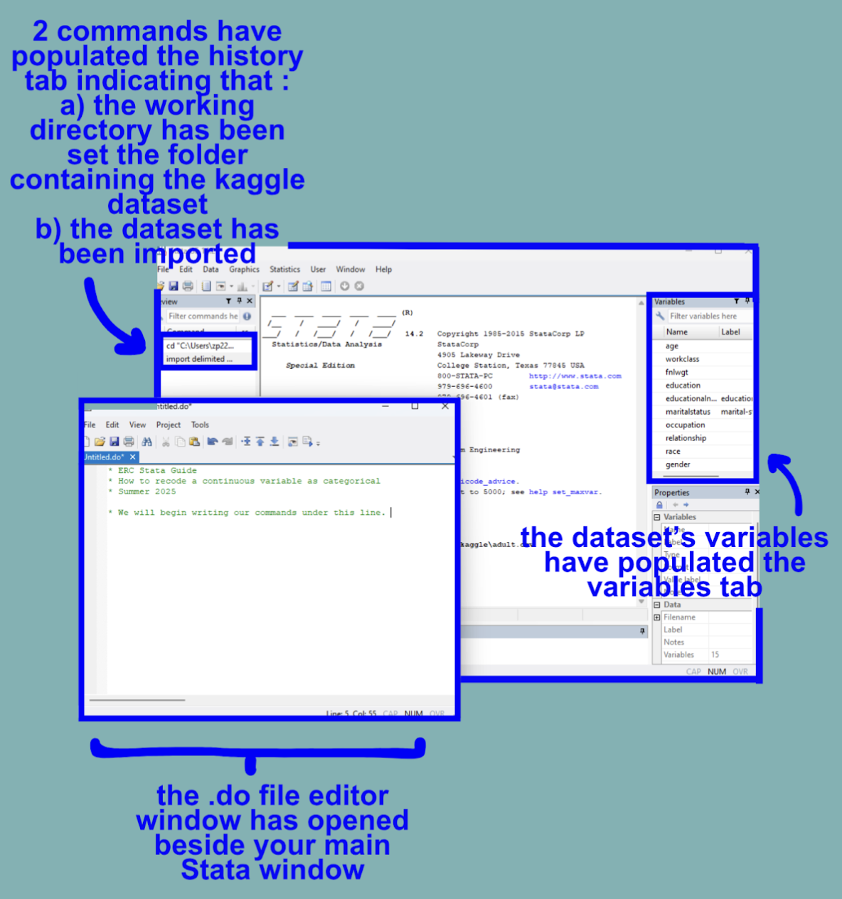
Once the initial setup steps have been accomplished, we can move on to viewing the data.
This variable happens to be stored as a number so we can bypass encoding as numeric (see general Stata guide or Stata’s PDF on encoding).
Let’s observe the summary statistics of this variable by running summarize.
summarize age
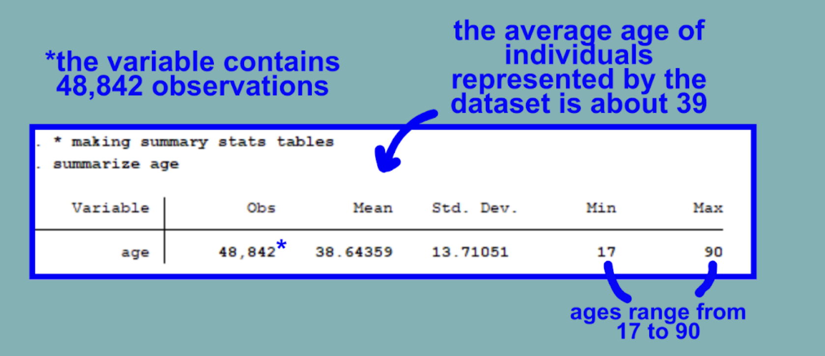
We can reference the census’ age groups to categorize our age variable in a similar way.
Let’s begin by making a new variable called agegroup where we’ll be categorizing the current continuous age variable as categorical.
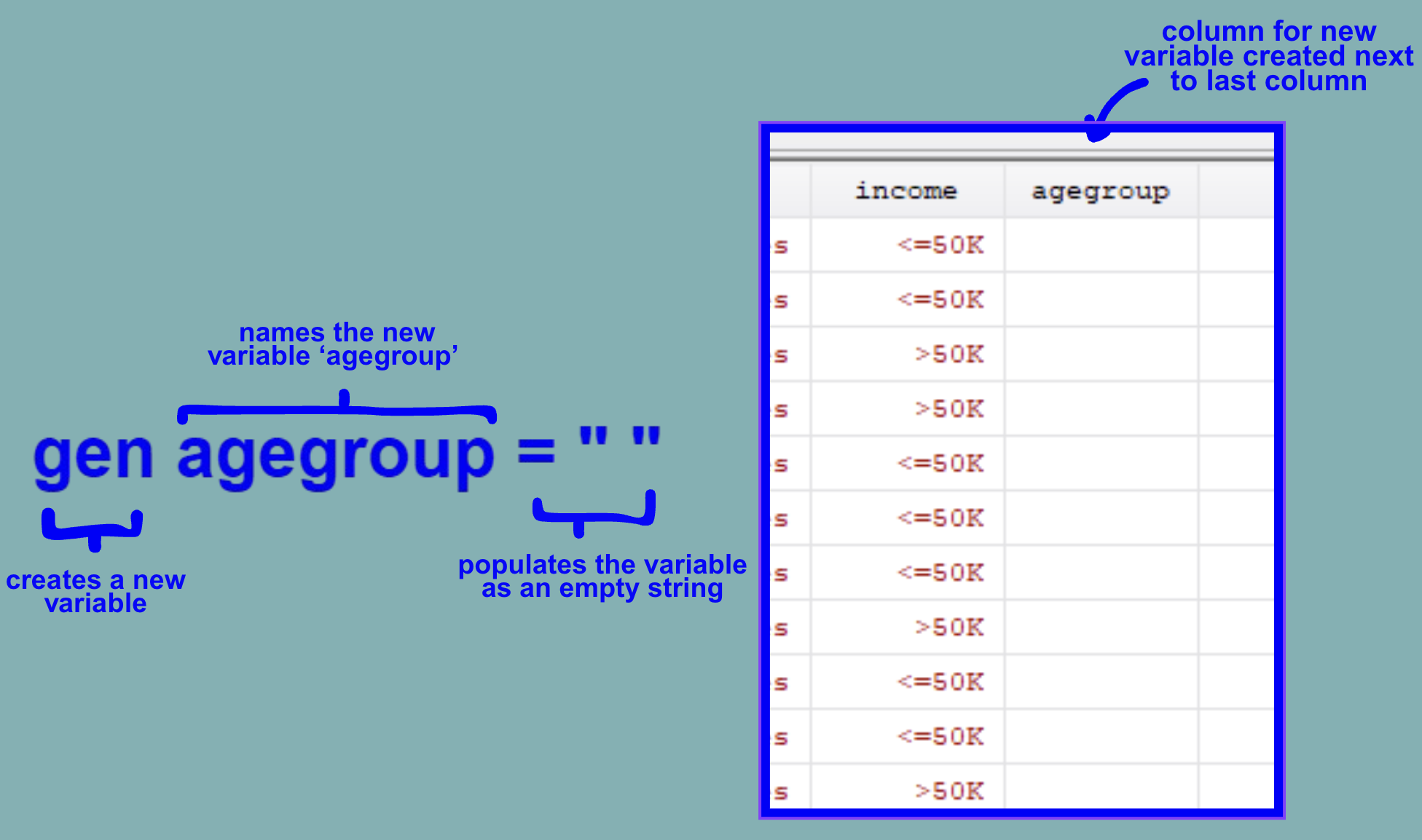
Now, let’s populate our new variable according to the 2020 census’ 9 age groups using either the replace command.

Each line follows the same intuition of replacing a cell of the agegroup variable with the respective category if the number under the continuous variable age falls within a certain bracket. The sorting process looks something like the image on the right:
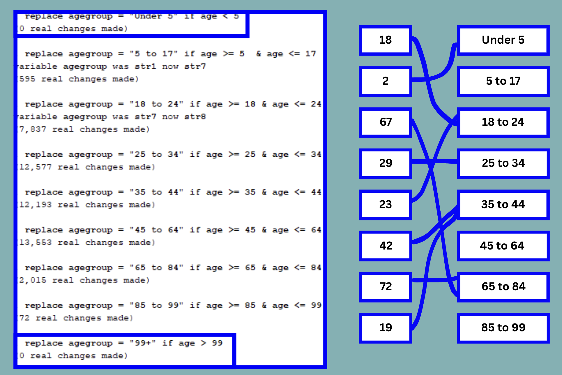
This is represented by the line under the two relevant commands which say, ‘0 real changes made’. We can observe that all other categories have been assigned respectively through the ‘real changes’ line or by browsing.
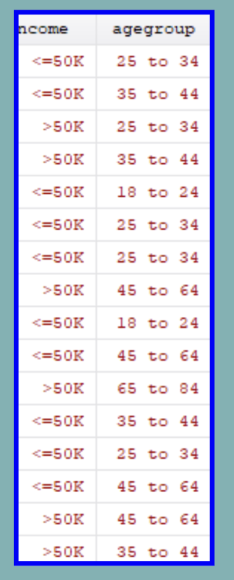
Use the browse command to view the results of reclassifying the variables.
You’ve now successfully reclassified a continuous variable as categorical! Continue reading to learn about two other kinds of intervariable classification!
II. Reclassifying between Categorical Variables
Reinterpreting a variable from one category to another is another usage of reclassifying. Taking our newly categorized agegroup variable from before*, we could reinterpret these age brackets to take on new meaning.
*If you are just interested in this section of the guide and haven’t completed the above, you may find an adjusted dataset for download (including the agegroup variable) here. to this section of the guide without.
We’ll now be looking at how to reclassify the age groups from above into the following categories:
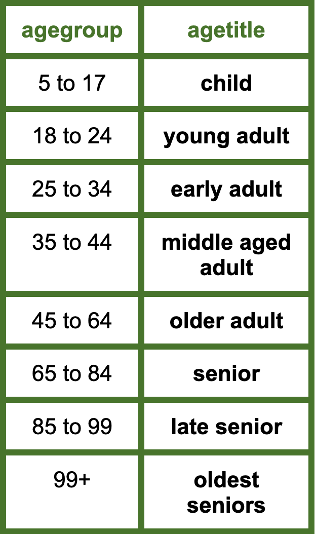
To do so let’s first create a new variable called agetitle by running the following:
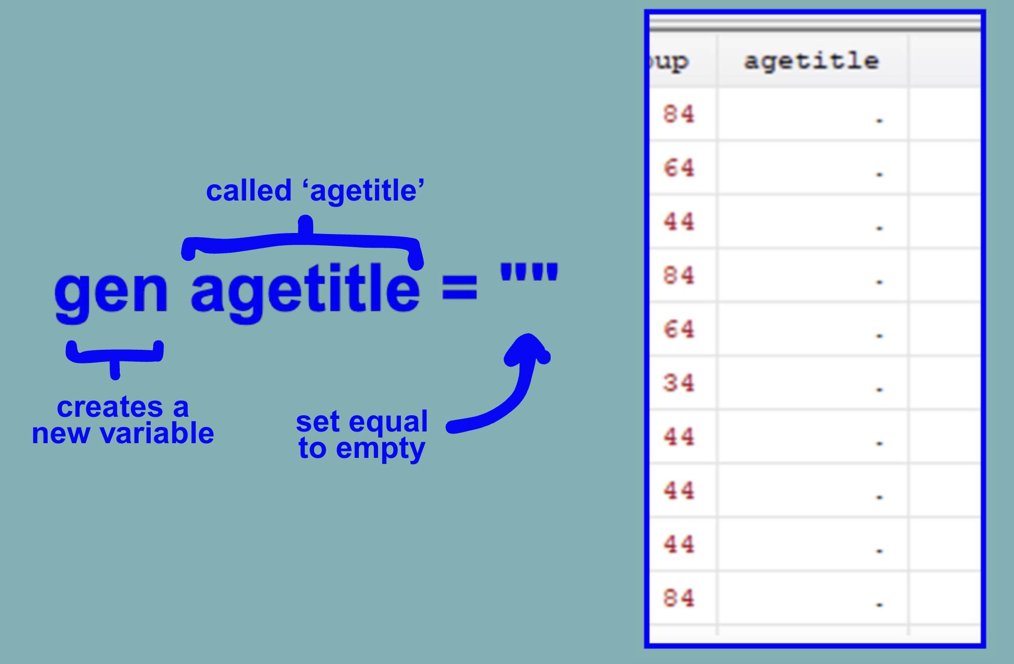
We can now move on to using the replace command to fill our new variable with equivalent title categories.

These commands follow the same logic as above where Stata checks if the agegroup variable fulfills a criteria (belonging to one of the categories), before replacing it with an equivalent category.

We can observe that the commands have successfully reclassified the age groupings into titles! Continue reading to learn about reclassifying categorical variables as binary ones.
III. How to Reclassify Variables as Binary
Another example of when it might be helpful to reclassify is when you would like to have a binary variable. Using our data from above, we might want to know simply if someone fulfills a certain criteria or not and code an observation as 0 or 1. Sometimes within your analysis, you will want to compare how one group reacts in comparison to all others.
Let’s reclassify the race variable as 1 if the respondent is indicated ‘Black’ or 0 if indicated any other race.
First, let’s check all the different categories represented under the race variable in our dataset by using the tab command:
tab race

We can now see the five different options for observations held under this variable.
Let’s now make a new variable called race_num to hold our numeric equivalents:

To reclassify the zeros and ones we’ll run: ![]()
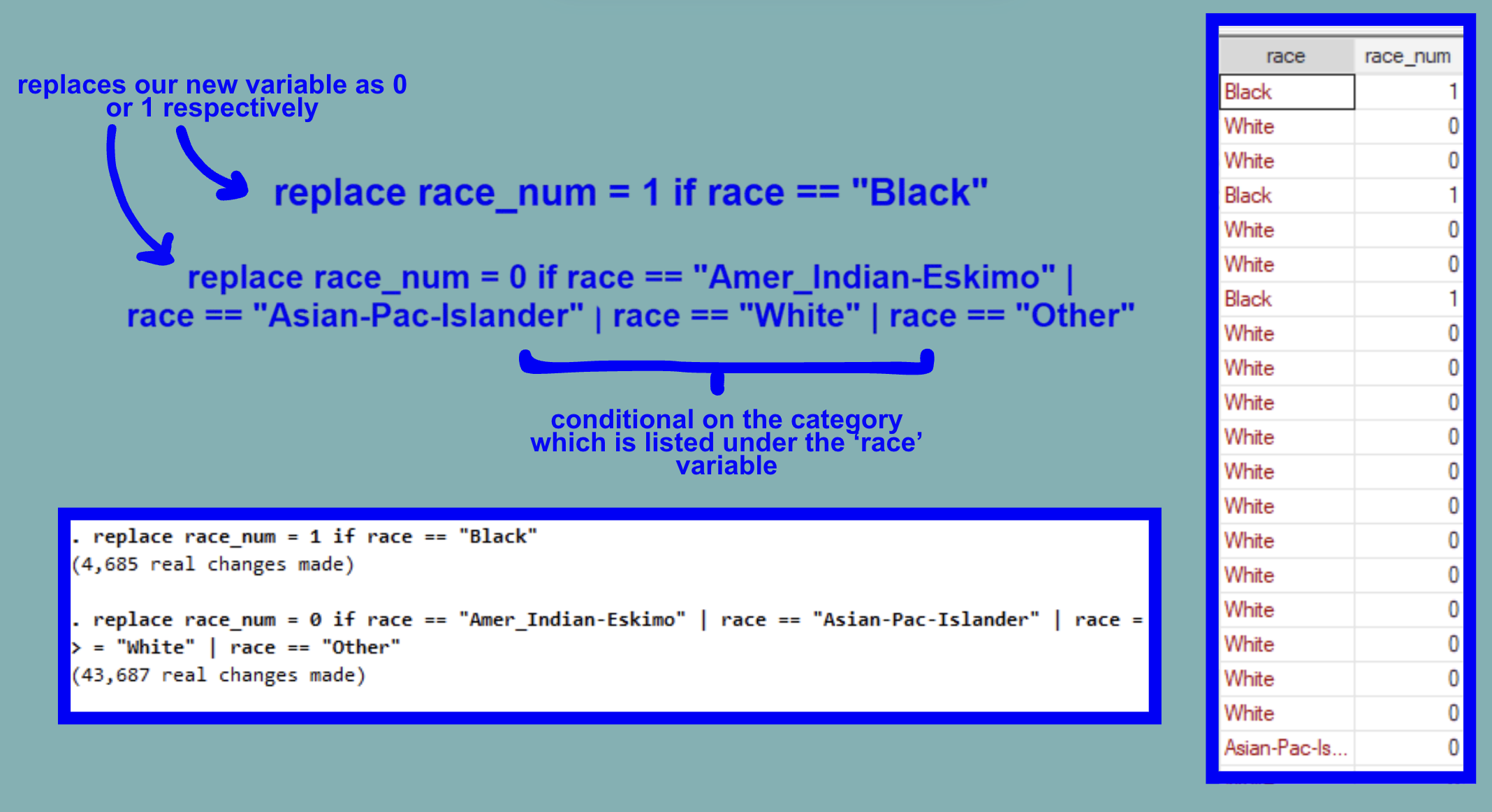
We can now see the successful output of the command under the race_num variable. Reclassifying the race variable has broadened the possibilities for types of analyses that might be ran.
Congrats on making it to the end of this ERC Stata How-To Guide!
For more How-Tos on using Stata see here:
- How to: Create Multiplots in Stata
- How to: Clean Survey Data in Stata
- How to: Append and Merge Data in Stata
- How to: Use Multiple Frames in Stata