Getting started with data analysis & visualization in Stata

What is ?

Stata is a statistical software used for data manipulation, visualization, and statistics, and can be helpful for exploring, summarizing, and analyzing datasets.

Stata operates through commands, or instructions for manipulating data. Common commands function to summarize data, create new variables, and run statistical testing. Commands in Stata can be run through the command tab at the bottom of the software or through a Do file (ending .do) which can be exported and saved for future reference.

If you are interested in running the commands as you follow along, the .do file including everything covered below can be found here.

Stata recognizes two main data types: Numeric and String.

★ Numeric variables: can be measured, represent numbers, and can be used in calculations

★ String variables: consist of characters and are not computable

The following will be covered within this guide:

I. Beginning Work in Stata

Downloading STATA and Workshop Materials

STATA is a paid software that requires a license for use. There is a student discount, but no free student version of the software. There are some locations on campus that have STATA downloaded and are free for students to use.

Where to find STATA licenses on campus:

★ Barnard’s Empirical Reasoning Center (Milstein 102)

★ Columbia Library Computers (various locations) **

** check Stata availability under the section of “Software in CUIT Computer Labs and Clusters”

Stata can be accessed remotely without downloading via Barnard’s Apporto or through Columbia’s virtual lab access services.

Here are the links to install Stata on your device:

Windows: Install on Windows

Mac: Install on Mac

You can also access Stata without having to download the software by using Apporto , a virtual computer lab through a web browser that you can access with your Barnard login.

For this guide, we will be working on a dataset of Student Performance & Behavior from Kaggle: https://www.kaggle.com/datasets/mahmoudelhemaly/students-grading-dataset?resource=download

After downloading the data into a zip file:

If using Windows: press Extract All
If using Mac: double click on the file

How to set up a Working Directory

A working directory is where STATA looks for all your files, it is whatever folder Stata thinks you're in. STATA will only be able to run on any data or documents within the working directory. Ensure that all the files you will be using are in the same working directory.

There are many ways to set up a working directory. For this workshop, we will define our working directory as the folder where our downloaded dataset is located. Once downloaded , the Kaggle dataset will likely be in your Downloads folder, but it is good practice to check the location of your files anyways so you know where they are when you load them on a data software like Stata ! To manually set up the directory through the software:

File → Change Working Directory → Downloads → **your folder name**

General Guidelines for Importing Data

STATA can work with one dataset at a time. A working directory must be set up before importing data that might come in different data file types: Sas, Csv, Excel, Txt, etc.

File → Import → **data file type you are working with**

The data set we will be using in this guide is in a CSV format. When you import a data file to stata to run an analysis, you need to specify the format of the data (.csv, .xls, .sas7bdat, .etc) you are importing when you select file → Import. To correctly import our .csv sample dataset from Kaggle, we specify :

Import→ Text data

Importing Data (.dta file)

In some cases, your data set might come as a .dta file. To load in a .dta file into your environment, select

File → Open

and select the .dta file you want to open.

Opening/Creating a .do File

A .do file is a code document where you can write and store a sequence of commands that process and analyse your data. A .do file allows the user to save commands and open them up later; this is convenient when picking up on a project later, or to share your code with someone.

If you would like to create a new .do file, go to the Window heading, go under Do-file-Editor and click New Do-file Editor.

Window → Do-file Editor → New Do-file Editor

Once the Do-file Editor is opened, you will be in an untitled .do file, where you can now put in your code. If your assignment or project requires you to use an existing Stata script, you can also open an existing .do file. To do this, select

File → Open → select .do file

Running commands in .do File

When you write code in the .do file, you are essentially writing instructions and steps for the program to complete. For these instructions to be carried out by your computer, you need to “run” or “execute” your code. When you run the commands in the Do-file Editor, they will be executed in the main Stata program.

It is good practice to run your code as you develop your script to make sure your program is running

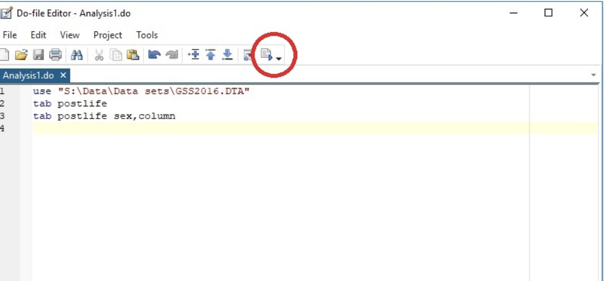
There are multiple ways to run your code within Stata: To run all commands in the .do file, click the rightmost icon (page with a play button). If you hover over the icon, it will say Execute(do). The Execute function instructs Stata to execute the commands stored in that file.

If you only want to run select lines of code: highlight the lines you want to run and select:

Tools→Execute(include)

Tabulating Variables

Now that the STATA environment has been set up, you can interact with the data.

For this specific dataset, we will be exploring how mental factors impact students' final scores.

View data

Before we start analyzing our data, we should look at the data. On the right hand side you can see all of your variables and their labels. When you select a variable, you can get more information on it in the Properties section, such as the data type.This can also be seen with the browse command. In the command line or your .do file, write browse. This opens a pop up with your data displayed as a spreadsheet with rows and columns, as well as the variable and properties section.

You can also deselect the checkboxes for specific variables on the left, so you can remove it from the dataset. This can help with refining your data to only the variables you will use.

We will focus on the sleep_hours_per_night, stress_level110, and final_score variables.

We can start off by tabulating our data. Tabulating a variable creates a frequency table of all the different values that a variable takes on and the corresponding number of observations.

tab sleep_hours_per_night

tab stress_level110

tab final_score

We can rename variables with the rename command. The rename command takes the existing variable name, followed by what you want to rename it to.

rename sleep_hours_per_night sleep

This command renames sleep_hours_per_night to sleep. Pay attention to spaces as they differentiate the variables.

rename stress_level110 stress

If you look at the variables list, you can see that the name of the variables have been updated. However, we can see that the label to the right still has the original name. We can change the label names to match the variable names. We use the label variable command followed by the name of the variable and what we want to change the label to

label variable sleep "sleep"

label variable stress "stress"

Now if we tabulate the stress variable, the label in the top left corner has changed to stress.

We can also cross tabulate two variables.This done with tab command followed by the two variables you want to tabulate.

tab stress sleep

If you would like to add the row and column percentages to a cross tabulation, you can run the following command.

tab stress sleep, row column

There is a key that tells you the first value is the frequency, the second is the row percentage and the third is the column percentage.

We can also get more information on a variable with the sum and codebook commands. The codebook command tells you the data type of the specified variable as well as missing values.

The tabstat command is an alternative way to get summary statistics and to select what you want. The command should be followed by the variable you want to summarize and the stats you want.

tabstat stress, stat(mean sd)

This command would give us the mean and standard deviation for the stress variable.

We can see that there are no missing values here. When you use your own datasets, there may be missing values, labelled as NA. This would automatically make a numeric value a string and mess up your data. We could fix this issue by converting all instances of NA to an empty string. This can be done with the following command, which works with string variables.

replace department ="" if department =="NA"

In this instance there were no NA values, but if there were, it would tell you how many instances there were and changed into an empty string.

If there are any variables that were intended to be numeric but were turned into strings because of the NA values, you can turn it back into a numeric data type with the following command. The workshop dataset does not have any instances of this, so we will use any string variable for demonstration.

destring department, replace

We can also analyse subsets of our data with the if command.

tab final_score if stress==7

This command tabulates the final when students’ stress levels were reported as 7. We can see the frequency of each test score. We can also tabulate this variable for all stress levels separately with the bysort command.

bysort stress: tab final_score

We can also use tabstat to choose the stats we want to run for final scores by stress levels

tabstat final_score, stat(mean sd) by(stress)

Using these tabulations, we can compare frequencies to see how stress affects final scores.

We can see that stress doesn’t have that great of an effect on final scores, but the highest average final scores are reported when the students had a stress level around 8.

As of now, we can see that the final scores are all tabulated distinctly by every two decimal spaces. We can create ranges for the variable so that it is easier to read.

egen final_score_ranges = cut(final_score), at(10,20,30,40,50,60,70,80,90,100)

This has created ranges for the final score and placed them into a new variable called final_score_ranges. We would also have to adjust the names to reflect the ranges.

Let’s say we also want to do analysis based on if a student got the recommended amount of sleep. We can recode the sleep variable to be binary; 1 will represent that they got enough sleep, and 0 will represent that they did not get enough sleep.

recode sleep (1/6.9=0) (7/10=1), generate(rec_sleep)

This recodes the sleep variable and takes all sleep hours from 1 through 6.9 and sets it to 0, indicating that they did not get enough sleep. It also takes the sleep hours between 7/10 and sets it to 1, indicating that they got enough sleep. This reading is stored in a new variable called rec_sleep.

We can see that rec_sleep only consists of 1’s and 0’s. The variables list also states that it is a recode of the sleep variable.

If we wanted to create a new variable called quiz_scores, we could run the following command.

gen quiz_scores =.

Data Analysis

Now that we have processed our data, we can do some analysis and data visualizations.

Let’s first run a correlation to observe the relationship between stress and students’ final scores.

We can see that stress and final scores are negatively correlated, so as stress increases, scores tend to decrease; however, it is a very weak correlation as it is close to 0.

We can also visualize the relationship of the two variables by creating a two way scatter plot of average sleep on average final score. To do this, we first have to calculate averages for final scores across all the sleep ratings. This can be done with the bysort command.

bysort sleep: egen avgscore=mean(final_score)

Now we can create a scatter plot between sleep and the average final scores. A two way scatter lists the variable on the y-axis followed by the variable on the x-axis.

graph twoway scatter avgscore sleep

We can also add a line of best fit with the following command:

graph twoway scatter avgscore sleep || lfit avgscore sleep

We can also run a linear regression, which helps us to get specific parameter estimates for our independent variables.

The regression command states the dependent variable followed by the independent variable(s). The following runs a regression to see how sleep affects final scores:

reg final_score sleep

This regression shows us that if the sleep changes by one unit, the final score is estimated to increase by .133. We can also see that the p-value is equal to .425, which means that this is not statistically significant.

You can create visualizations in STATA by either directly writing the code with relevant commands, or using the Graphics tab. We can start off by creating a histogram to see the distribution of the final scores.

By: Zoe Pyne