Getting started with regressions in R
In this guide we you will:
- Understand Variable Types in R
- Learn how to check or convert variable types in R.
- Learn how to code a simple and multiple linear regression.
- Interpret of regression output (coefficients, p-values, R-squared, and residuals).
This guide is designed to help you build confidence in reading and interpreting regression results in R. Whether you're a beginner or refreshing your understanding, this walkthrough will clarify how to interpret key regression outputs like coefficients, p-values, R-squared, and their residuals, and explain what they tell us about the relationships between variables. We'll walk through both simple and multiple linear regressions, starting with built-in datasets like “ChickWeight” exploring the relationship between chick weight (gm) and time (days) and then moving onto an economic dataset using the wooldridge package. Along the way, you'll learn :- Understand Variable Types in R
- Learn how to check or convert variable types in R.
- Learn how to code a simple and multiple linear regression.
- Interpret of regression output (coefficients, p-values, R-squared, and residuals).
- How R handles different types of variables
- How to recognize which are treated as categorical or numeric
- How to interpret the effects of each predictor variable
- How to interpret control variables
Understanding Variable Types in R
Before diving into our first dataset, “ChickWeight,” and analyzing the effect of time on chick weight, it’s essential to first understand the types of variables we're working with. In R, variable types matter a lot. R treats different types of variables differently in analyses, visualizations, and even in basic summaries. Knowing this allows you to avoid errors in models, interpret results correctly and choose the right functions or plots. We will break down all types for you
R Divides variables into two main groups:
| Category | Description |
|---|---|
| Categorical (Qualitative) | Represents groups or labels—not numbers |
| Numerical (Quantitative) | Represents measurable quantities |
By labels we refer to values that categorize observations into distinct groups, such as "Male" and "Female" for gender, or "Diet 1", "Diet 2", "Diet 3" for different treatment types of food. These labels do not represent numeric magnitude or order (unless specifically defined as ordered), but instead serve to group or differentiate cases in the dataset.
Each of these is stored in different data types, which tells R how to handle them.
| Type | What It Is | Stored As | Example |
|---|---|---|---|
| Nominal | Categories with no order | Factor (helps R understand variables as categories, not as values with numeric meaning) | City, Diet type |
| Ordinal | Categories with a hierarchy Ordered categories |
ordered factor | Education level |
| Binary | Two categories only (Yes/No, 0/1) | factor or logical | Voted (Yes/No) |
| Character | Text labels (non-categorical) | character | Names, Email |
NOTE: In R, a factor is a special data type used to indicate that a variable represents categories, not numerical values.
This tells R to treat the variable as a set of labels or groups rather than quantities.
As observed above, some of those have no order, such as having variables for cities or provinces like “New York”, “San Francisco”, “Seattle”, etc.
And some, although not numerical, pertain to a certain order in their category—such as education, where we know lower school comes before middle school, high school, and college.
In R numerical values are understood in the following manner,
| Type | What It Is | How R Treats It | Use Case |
|---|---|---|---|
| Continuous | Any value (e.g., 23.4, 102.7) | numeric | Use in regression, plots |
| Discrete | Whole counts (e.g., children = 3) | integer/numeric | Sometimes modeled as counts |
| Proportions | 0–1 or 0–100 (e.g., % complete) | numeric | Can use as is or transform |
| Counts | How many times something happened | integer | Often used in Poisson models |
How R Treats These in Modeling,
| Variable Type | Used in Regressions? | Interpreted As |
|---|---|---|
| factor | Yes | Dummy variables vs. reference group |
| ordered factor | Yes (less common) | Can use contrasts for trends |
| character | No | Must convert to factor first |
| numeric/integer | Yes | Continuous predictor |
| logical | Yes (TRUE = 1, FALSE = 0) | Binary predictor |
How to Check or Convert Variable Types in R.
Sometimes, R doesn't automatically recognize a variable the way you intend. For example, you might have text stored as characters when it should be treated as categories, or numbers that represent levels (like education) that should be ordered, not treated as continuous quantities. As a result, you must help R “understand” your data by giving it the right label, so it doesn't misinterpret it when running models or making plots.
This quick example shows you how to check and convert each variable type
This quick example shows you how to check and convert each variable type
R
# Check variable structure
str(data1)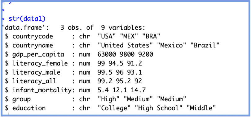
R
# Convert character to factor
data$group <- as.factor(data$group)

# Convert numeric to ordered factor
data$education <- factor(data$education,
                         levels = c("Primary", "Middle", "High School", "College"),
                         ordered = TRUE)

# Convert factor back to numeric (if needed)
as.numeric(as.character(data$factor_var)) 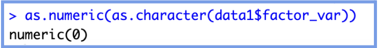
Understanding these conversions is crucial as it ensures your model makes sense, your plots are accurate and R won't misinterpret numbers as quantitative when they are just labels.
What is a regression?
Regressions are one of the most widely used tools in data analysis. They help us understand how one variable relates to another, and allow us to predict outcomes using known inputs.
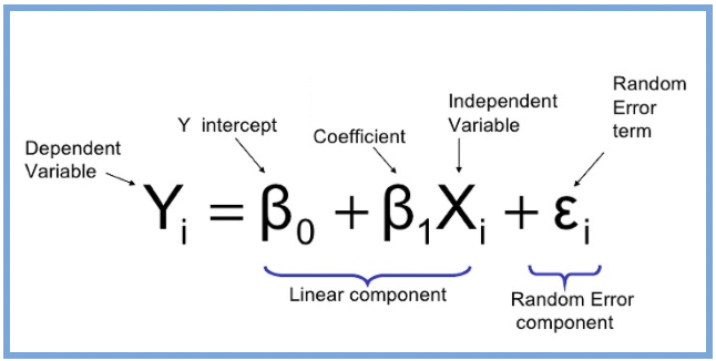
At its core, a regression is a way to model the relationship between:
- One outcome variable (also called the dependent variable or Y)
- And the one or more predictor variables (called the independent variables or X)
In R:
model <- lm() # fit linear model
Inside the parenthesis: goal(y ~ x, data = mydata)
This line tells R to fit a linear model where:
model <- lm() # fit linear model
Inside the parenthesis: goal(y ~ x, data = mydata)
This line tells R to fit a linear model where:
- y is the dependent (outcome) variable
- x is the independent (predictor) variable
- mydata is the name of your dataset
We will perform a deep dive into each of the above metrics and how to read them, with the goal of understanding what each metric is telling us about the model. To do this we 'll be using a data set that is already built into R called “ChickenWeight”. This data set has 578 rows and 4 columns, from an experiment on the effect of diet on early growth of chicks. To start, we will be investigating the relationship between chick weight (gm) and time (days) asking: How does the weight of a chick change over time?
This code allows you to see and understand the data set:
This code allows you to see and understand the data set:
R
# Load built-in dataset
data(ChickWeight)

# View the first few rows
head(ChickWeight)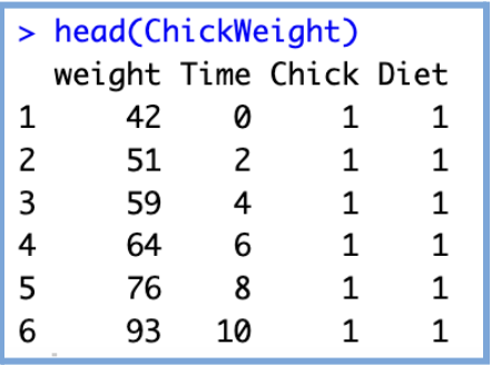
R
# View variable names
names(ChickWeight)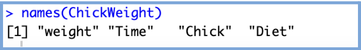
Variables:
- weight: a numeric vector giving the body weight of the chick (gm). (continuous numerical)
- Time: a numeric vector giving the number of days since birth when the measurement was made. (discrete numerical that acts as continuous)
- Chick: an ordered factor with levels 18 < … < 48 giving a unique identifier for the chick. The ordering of the levels groups chicks on the same diet together and orders them according to their final weight (lightest to heaviest) within the diet. (Categorical, ordinal Identifier)
- Diet: a factor with levels 1, …, 4 indicating which experimental diet the chick received. (Categorical Nominal)
R
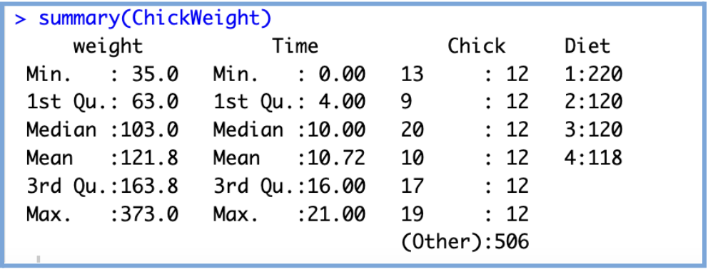
# Structure of the dataset
str(ChickWeight)

# Summary statistics
summary(ChickWeight)
This provides basic descriptive statistics for each variable in the dataset, including the minimum, maximum, mean, median, as well as the 1st and 3rd quartiles. These values give you a quick sense of the data’s distribution, central tendency, and spread, which helps us identify outliers, skewed variables, or potential issues before modeling.
How to Run a Simple Linear Regression in R
We’ll start by running a simple regression model with time as our dependent variable and chicken weight (gm) as our independent variable. The code and the output of this regression model are below. The simple regression model is achieved by using the lm() function in R and the output is called using the summary() function on the model.
REMINDER: R is case-sensitive! Variables like
Weight, weight, and WEIGHT are treated as completely different.
Make sure to use the exact variable names (you can check them using names(ChickWeight) or str(ChickWeight))
because calling on the wrong variable name will lead to an error.
R
model1 <- lm(weight ~ Time, data = ChickWeight)
summary(model1)
Output:
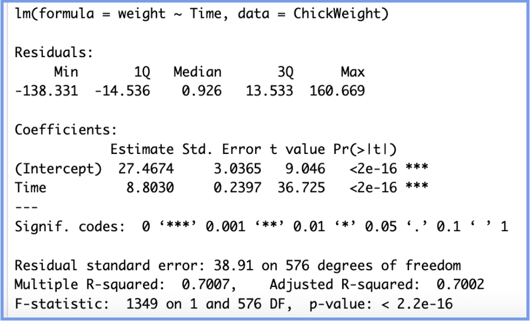
Now that we have a model and output, let's walk through each part of the model step by step so we can better understand each section and how it helps us determine the effectiveness of the model.
CALL
The call section shows us the formula that R used to fit the regression model, weight is our dependent variable and we are using Time as a predictor (independent variable) from the data set ChickenWeight.
COEFFICIENTS
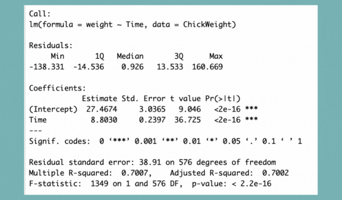
The next section in the model output talks about the coefficients of the model. We are looking to build a generalized model in the form of the slope equation, y=mx+b, where b is the intercept and m is the slope of the line. Because we often don’t have enough information or data to know the exact equation that exists in the wild, we have to build this equation by generating estimates for both the slope and the intercept. These estimates are most often generated through the ordinary least squares method (OLS), which is a fancy way of saying that the regression model finds the line that fits the points in such a way that it minimizes the distance between each point and the line (minimizes the sum of the squared differences between the actual values and the predicted values).
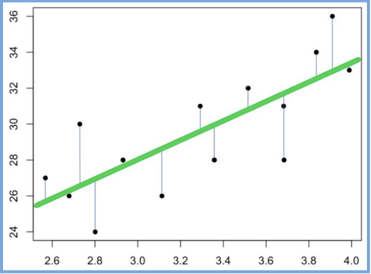
The line above is a visual representation of how we obtain our coefficients. The point at which the line meets the y-axis is our intercept (b) and the slope is our (m). With this we can build our model equation:
Predicted Weight=27.47+8.80×Time
How do we interpret each estimate? The (intercept) can be interpreted as follows: when Time=0, a chick weighs 27.47 grams, in other words, when born (time =0) a chick will weigh 27.47 grams on average.
The Time estimate can be interpreted as follows:On average, for each additional day, a chick gains about 8.80 grams of weight.
The standard error of the coefficient is an estimate of the standard deviation of the coefficient. In effect, it is telling us how much uncertainty there is with our coefficient. The standard error is often used to create confidence intervals. For example we can make a 95% confidence interval around our slope by multiplying by 1.96, time:
8.8030±1.96(0.2397)=(8.3334, 9.2726)
Looking at the confidence interval, we can say that we are 95% confident the actual slope is between 8.33 and 9.27.
Apart from being helpful for computing confidence intervals and t-values, this is also a quick check for significance. If the coefficient is large in comparison to the standard error, the confidence interval will not include zero—which suggests the coefficient is statistically significant. In our case, since the interval does not include 0, we can confidently say that time has a significant positive effect on chick weight.
The t-statistic is simply the coefficient divided by the standard error. In general, we want our coefficients to have large t-statistics, because that indicates the standard error is small relative to the estimate, meaning our estimate is more precise. Simply put, the t-statistic tells us how many standard errors away from zero the coefficient is.
In our example, the coefficient for Time is 36.73 standard errors away from zero, which is extremely far in statistical terms. The larger the t-statistic, the more confident we are that the coefficient is not zero, i.e., that it represents a real effect. The t-statistic is then used to calculate the p-value, which helps us determine the statistical significance of the coefficient.
In the regression output, the Pr(>|t|) column shows the p-value for each coefficient. This represents the probability of observing a t-statistic as extreme as the one calculated, assuming the null hypothesis is true (i.e., assuming the true coefficient is 0). In simple terms, we ask: “if there is no relationship, what are the chances we'd get a t-value this big?” Small p-values (typically < 0.05) suggest that the observed relationship is unlikely to be due to chance. A small p-value allows us to reject the null hypothesis and conclude that the coefficient likely represents a real effect.
In our model, the p-value for both the intercept and Time is less than than 2e-16, which is essentially zero. This is marked by three asterisks (***) indicating a high level of statistical significance. So we can say that the time coefficient is highly significant, confirming a strong relationship between time and weight. Every day, chicks gain approximately 8.80g, and this growth rate is very unlikely to be due to random variation.
The Time estimate can be interpreted as follows:On average, for each additional day, a chick gains about 8.80 grams of weight.
Coefficients - Std. Error
The standard error of the coefficient is an estimate of the standard deviation of the coefficient. In effect, it is telling us how much uncertainty there is with our coefficient. The standard error is often used to create confidence intervals. For example we can make a 95% confidence interval around our slope by multiplying by 1.96, time:
8.8030±1.96(0.2397)=(8.3334, 9.2726)
Looking at the confidence interval, we can say that we are 95% confident the actual slope is between 8.33 and 9.27.
Apart from being helpful for computing confidence intervals and t-values, this is also a quick check for significance. If the coefficient is large in comparison to the standard error, the confidence interval will not include zero—which suggests the coefficient is statistically significant. In our case, since the interval does not include 0, we can confidently say that time has a significant positive effect on chick weight.
Coefficients - t-value
The t-statistic is simply the coefficient divided by the standard error. In general, we want our coefficients to have large t-statistics, because that indicates the standard error is small relative to the estimate, meaning our estimate is more precise. Simply put, the t-statistic tells us how many standard errors away from zero the coefficient is.
In our example, the coefficient for Time is 36.73 standard errors away from zero, which is extremely far in statistical terms. The larger the t-statistic, the more confident we are that the coefficient is not zero, i.e., that it represents a real effect. The t-statistic is then used to calculate the p-value, which helps us determine the statistical significance of the coefficient.
Coefficients – Pr(>|t|) and significance
In the regression output, the Pr(>|t|) column shows the p-value for each coefficient. This represents the probability of observing a t-statistic as extreme as the one calculated, assuming the null hypothesis is true (i.e., assuming the true coefficient is 0). In simple terms, we ask: “if there is no relationship, what are the chances we'd get a t-value this big?” Small p-values (typically < 0.05) suggest that the observed relationship is unlikely to be due to chance. A small p-value allows us to reject the null hypothesis and conclude that the coefficient likely represents a real effect.
In our model, the p-value for both the intercept and Time is less than than 2e-16, which is essentially zero. This is marked by three asterisks (***) indicating a high level of statistical significance. So we can say that the time coefficient is highly significant, confirming a strong relationship between time and weight. Every day, chicks gain approximately 8.80g, and this growth rate is very unlikely to be due to random variation.
RESIDUALS
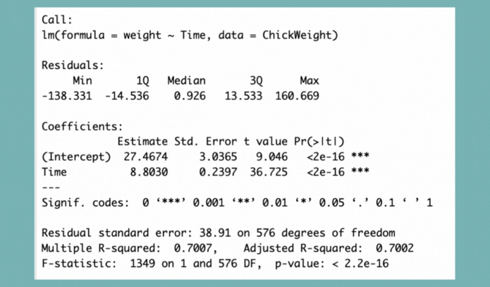
The residuals are the difference between the actual values and the predicted values.
So how do we interpret this? Well, thinking critically about it, we’d definitely want our median value to be centered around zero as this would tell us that our residuals were somewhat symmetrical. This also means that our model was predicting evenly at both the high and low ends of our dataset. When we look at our residuals, the fact that our median is greater than zero suggests that our model is slightly rightly skewed. This tells us that our model is not predicting as well at the higher weight ranges as it does for the lower ones. In other words, some chicks' weights are underpredicted—especially those on the heavier end.
So how do we interpret this? Well, thinking critically about it, we’d definitely want our median value to be centered around zero as this would tell us that our residuals were somewhat symmetrical. This also means that our model was predicting evenly at both the high and low ends of our dataset. When we look at our residuals, the fact that our median is greater than zero suggests that our model is slightly rightly skewed. This tells us that our model is not predicting as well at the higher weight ranges as it does for the lower ones. In other words, some chicks' weights are underpredicted—especially those on the heavier end.
RESIDUAL STANDARD ERRORS
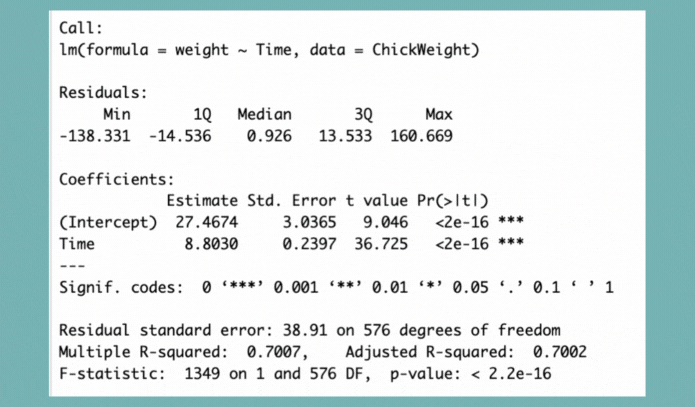
The Residual Standard Error (RSE) is a measure of the quality of a linear regression fit. In theory, every linear model includes an error term (ε), which accounts for the variation in the response variable that is not explained by the predictor(s). Because of this error term, our predictions won’t perfectly match the observed values. The RSE represents the average amount that the observed values deviate from the regression line. In our example, the actual chick weights deviate from the predicted regression line by about 38.91 grams, on average. In other words, even though our model explains a substantial portion of the variation in weight (as shown by the high R²), any individual prediction is still expected to be off by about 38.91 grams on average.
It’s also worth noting that the Residual Standard Error was calculated with 576 degrees of freedom. Degrees of freedom reflect the number of independent data points used to estimate the model after accounting for the number of parameters estimated (in our case, the intercept and the slope). In our case, we had 578 observations and two parameters.
It’s also worth noting that the Residual Standard Error was calculated with 576 degrees of freedom. Degrees of freedom reflect the number of independent data points used to estimate the model after accounting for the number of parameters estimated (in our case, the intercept and the slope). In our case, we had 578 observations and two parameters.
R-SQUARED
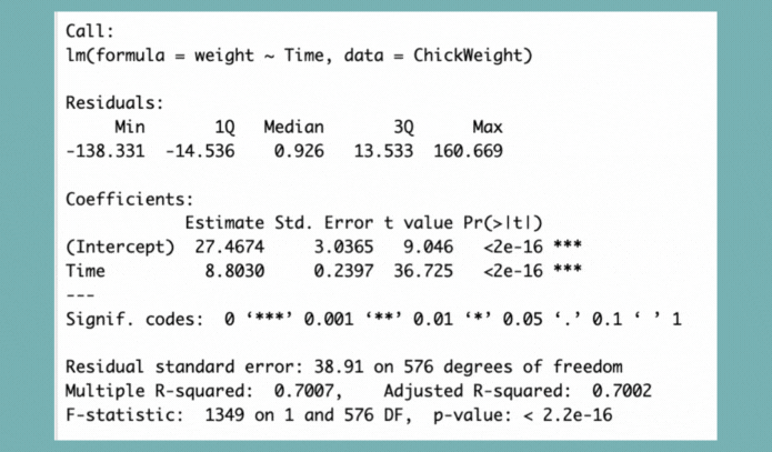
The R-squared (R²) statistic provides a measure of how well the model fits the actual data. It represents the proportion of variance in the response variable that is explained by the predictor(s). R² values range from 0 to 1, where:
In our example, the Multiple R-squared is 0.7007. This means that approximately 70% of the variation in chick weight can be explained by the variable Time. That’s a fairly strong relationship, especially considering we’re using only one predictor. Think about it: if you were trying to predict a chick’s weight, wouldn’t age (time) be one of the most important variables? It makes intuitive sense that as chicks get older, they gain weight, so it’s not surprising that Time is a strong predictor.
That said, it’s always important to note that what constitutes a "good" R² depends on the context. In some fields (like biology or economics), even an R² of 0.3 might be meaningful, while in others (like physics), 0.9 might be expected.
- A value near 0 means the model explains very little of the variation.
- A value near 1 means the model explains most of the variation.
In our example, the Multiple R-squared is 0.7007. This means that approximately 70% of the variation in chick weight can be explained by the variable Time. That’s a fairly strong relationship, especially considering we’re using only one predictor. Think about it: if you were trying to predict a chick’s weight, wouldn’t age (time) be one of the most important variables? It makes intuitive sense that as chicks get older, they gain weight, so it’s not surprising that Time is a strong predictor.
That said, it’s always important to note that what constitutes a "good" R² depends on the context. In some fields (like biology or economics), even an R² of 0.3 might be meaningful, while in others (like physics), 0.9 might be expected.
NOTE: In multiple regression settings, the “Multiple R-Squared” will always increase as more variables are
included in the model. That's why the adjusted R-squared is the preferred measure, as it adjusts for the number of variables considered.
F-STATISTIC
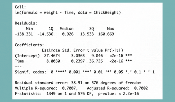
We can see from our model, the F-statistic is very large and our p-value is so small it is basically zero. This would lead us to reject the null hypothesis and conclude that there is strong evidence that a relationship does exist between chick weight and time.
Adding More Variables to the Regression
Once you've explored a simple linear regression (like predicting weight from time in the ChickWeight dataset), you’re ready to complicate the model by adding more predictors. This is called Multiple Linear Regression. When you include additional variables, these are often referred to as controls, they help you isolate the effect of your main predictor by accounting for other factors that might influence the outcome. In other words, you're holding other variables constant to better understand the unique contribution of each one.
To start, we will continue working with the built-in ChickWeight dataset. In this new model, we’ll include both Time and Diet (categorical with 4 levels) as predictors of weight.
R
model2 <- lm(weight ~ Time + Diet, data = ChickWeight)
summary(model2)
This is the output we obtain from running the code:
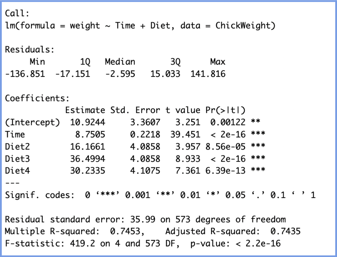
We will interpret the results in the following manner:
- Interpret (10.92): When Time = 0 (i.e., at birth) and the chick is on Diet 1 (the reference group), the expected weight is 10.92 grams. This is the baseline starting weight.
- NOTE: In regression models, a reference group is the baseline category used when a categorical variable is included in the model.Since regression models can only include numeric values, R (and most software) converts categorical variables into dummy variables (binary indicators (0 or 1) for each group). However, one group must be left out to avoid redundancy. This group becomes the reference group. In this case, Diet 1 becomes the reference group, and all other diet coefficients are interpreted in comparison to this reference group.
- Time (8.7505):
- Diet Coefficients (relative to Diet 1):
- Diet 2: On average, chicks on Diet 2 weigh 16.17g more than those on Diet 1, controlling for age.
- Diet 3: Chicks on Diet 3 weigh 36.50g more than those on Diet 1.
- Diet 4: Chicks on Diet 4 weigh 30.23g more than those on Diet 1.
All three differences are statistically significant (p < 0.001), indicating that diet type has a clear impact on weight.
Finally, through the R-squared values we can observe that our model explains 74.3% of the variation in chick weight. This is a very strong fit for biological data.
As a result, this multiple linear regression model shows that time since birth and diet type both have strong, statistically significant effects on chick weight. Chicks grow at a steady rate over time, and those on higher-numbered diets, especially Diet 3, tend to weigh more, even after controlling for age.
Now we can apply this same logic using a data set from the economics discipline called “bwght” from the Wooldridge package, which explores factors affecting birth weight.
As a result, this multiple linear regression model shows that time since birth and diet type both have strong, statistically significant effects on chick weight. Chicks grow at a steady rate over time, and those on higher-numbered diets, especially Diet 3, tend to weigh more, even after controlling for age.
Working With an Economics Data Set
Now we can apply this same logic using a data set from the economics discipline called “bwght” from the Wooldridge package, which explores factors affecting birth weight.
R
install.packages("wooldridge")
library(wooldridge)
data("bwght")
The dataset includes 1,388 observations on 14 variables from the 1988 National Health Interview Survey. Below are a few key variables:
| Variable | Meaning | Type |
|---|---|---|
| bwght | Birth weight (ounces) | Continuous numeric |
| famincome | 1988 family income ($1,000s) | Continuous numeric |
| cigs | Cigarettes smoked per day while pregnant | Discrete numeric |
| motheduc | Mother’s years of education | Ordinal numeric |
| white | =1 if white, 0 otherwise | Binary (factor/logical) |
Building a More Complex Linear Model:
Let’s build a multiple linear regression model to predict the impact of smoking cigarettes during pregnancy on infant birth weight (bwght), while controlling for other relevant factors. This allows us to isolate the effect of smoking from other variables that might also influence birth outcomes, such as mother’s education, income, or race.
R
model_bwght <- lm(bwght ~ cigs + motheduc + white + income, data = bwght)
summary(model_bwght)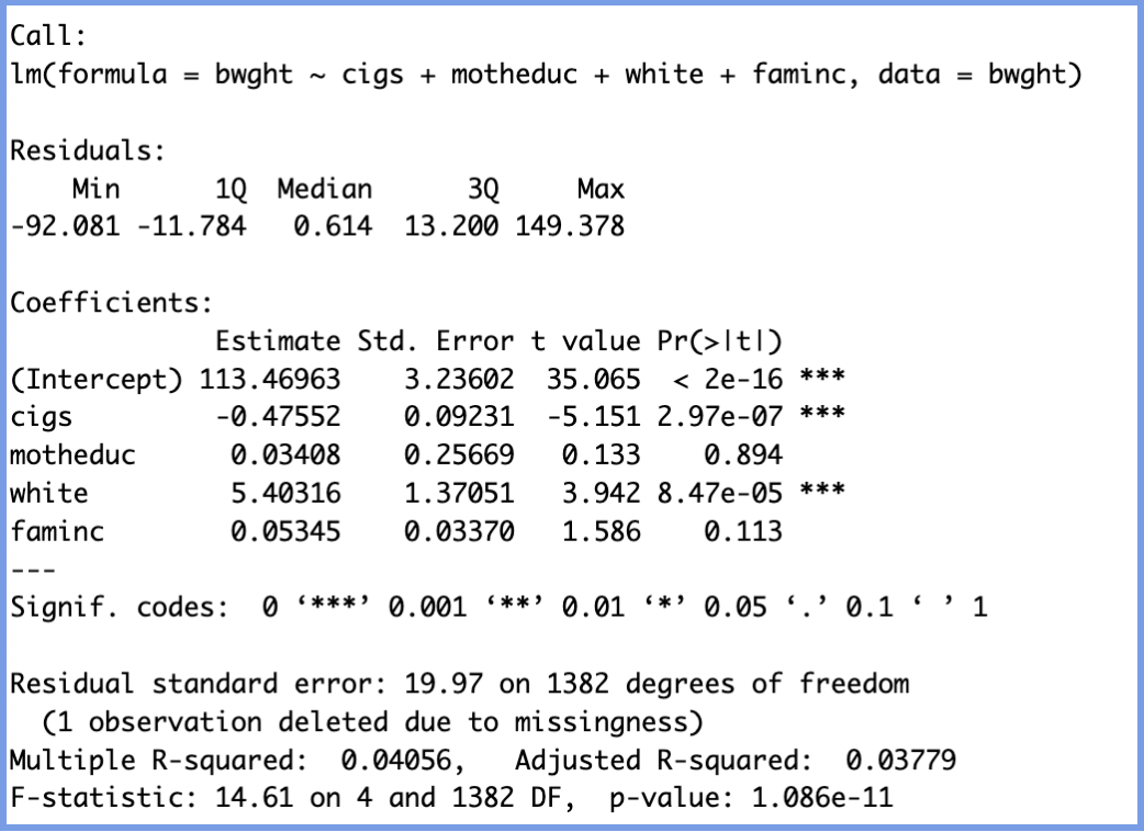
Once again, we will interpret the variables and understand the constants by examining both the magnitude and direction of each coefficient, while keeping in mind the effect of controlling for other variables in the model.
| Variable | Type | Coefficient | Interpretation | Statistical Significance |
|---|---|---|---|---|
| cigs | Continuous | −0.476 |
When controlling for a mother’s education, race, and income, each additional cigarette smoked per day is associated with a 0.48 oz decrease in birth weight. |
*** (p < 0.001) |
| motheduc | Continuous | +0.034 |
When controlling for smoking, race, and income, each additional year of mother’s education is associated with a 0.03 oz increase in birth weight. |
Not significant (p = 0.894) |
| white | Binary (Binary variables compare the presence vs. absence of a characteristic, e.g., white vs. other race) |
+5.403 |
When controlling for smoking, education, and income, being white is associated with a 5.4 oz increase in expected birth weight. |
*** (p < 0.001) |
| faminc | Continuous | +0.053 |
When controlling for smoking, education, and race, each additional $1,000 in family income is associated with a 0.05 oz increase in birth weight. |
Not significant (p = 0.113) |
Through this, we can observe that the biggest impacts on weight came from being white and smoking cigarettes, but while one decreased the weight by almost 0.5 ounces per cigarette the other one increased the weight by 5.40 pounds just because of race. Both of these effects are statistically significant (p < 0.001), suggesting they likely reflect real relationships rather than random variation. This underscores how certain social and behavioral factors can meaningfully influence the dependent variable—in this case, infant weight.
It’s also important to note that this model can be expanded to include additional relevant predictors in order to improve its explanatory power (as measured by the R-squared) and to capture more of the variation in the data. For example, we might consider including father’s education, a more detailed measure of smoking such as packs per day, or even factors like maternal age, prenatal care visits, or diet during pregnancy.
By: Sofia Covarrubias
It’s also important to note that this model can be expanded to include additional relevant predictors in order to improve its explanatory power (as measured by the R-squared) and to capture more of the variation in the data. For example, we might consider including father’s education, a more detailed measure of smoking such as packs per day, or even factors like maternal age, prenatal care visits, or diet during pregnancy.
Caveat: While adding more variables can enhance the model, it also comes with trade-offs.
Including too many predictors, especially those that are irrelevant or highly correlated with others, can lead to overfitting,
where the model captures noise rather than true patterns. This can reduce its accuracy when applied to new data.
Additionally, a more complex model can become harder to interpret and communicate clearly.
As mentioned before, it is important to always keep tabs on the adjusted R-squared for this analysis,
as it may not increase even when more variables are added.
Ultimately, each added variable has the potential to refine the model and deepen our understanding of the underlying dynamics. Thoughtful model expansion allows us to uncover more accurate and nuanced insights into the factors influencing birth weight.By: Sofia Covarrubias