How to Clean and Preprocess Survey Data in R Studio

Welcome to the R Guide on cleaning and preprocessing survey Data! Cleaning and preprocessing are crucial preliminary steps when conducting research which utilizes survey data.There are many elements of survey data which need to be adjusted before being able to successfully conduct relevant analyses.

Throughout this guide, blue phrases will be used to indicate commands, green phrases for variables, and purple for links and downloads.

We’ll be using an adjusted version of the first file from the National Health and Nutrition Examination Survey (NHANES). The link can be found here. The dataset contains a breadth of demographic information which we will be learning how to clean and preprocess.

Here is the R script which you can use to follow the guide with.

Begin by downloading the data, saving it to a folder, and loading the haven, tidyverse, and survey packages relevant to this guide.

library(haven)
library(tidyverse)
library(survey)

How is a Survey’s Design Specified?

The NHANES is a broad project which spans a variety of different surveys and topics. Its goal is to “assess the health and nutritional status of adults and children in the United States” (ICPSR, 2025). In the file of it that we’ve been using, we have four important variables related to the survey’s design and how it’s meant to be analyzed:

WTINT2YR: Full Sample 2 Year Interview Weight
WTMEC2YR: Full Sample 2 Year MEC Exam Weight
SDMVPSU: Masked Variance Pseudo - PSU
SDMVSTRA: Masked Variance Pseudo-Stratum

So, what do these mean and how do they allow us to specify something about the survey’s design?

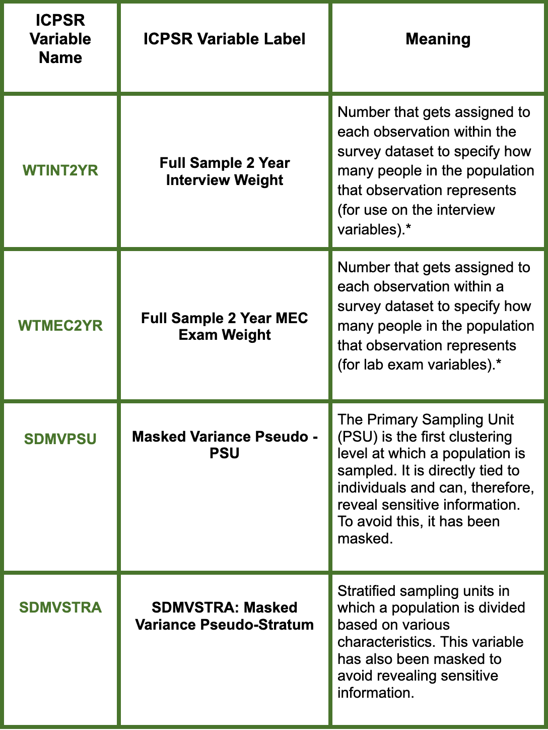
*WTINT2YR and WTMEC2YR are both sampling weights but while the first is to be used in relation to interview data, the second should be used for exam data. In our case, we will be focusing on WTINT2YR since the demographic variables have been collected through conducted interviews. WTMEC2YR is used on the elements of the survey which would need to be collected by a lab exam (i.e. blood glucose levels).

** Here is a small diagram from ‘Statistical Aid’ for help on visualizing the stages of sampling utilized within a survey’s sampling.

Now that we’ve learned about the four variables in the dataset related to the survey’s design, let’s use the appropriate ones to specify the survey characteristics in R.

We’ve now successfully adjusted the settings in R for the appropriate design specification. Stata can now appropriately implement the weighting and stratification information included from the NHANES. Let’s move on to cleaning the data.

Missing Values

Viewing the data in a spreadsheet (using the play button next to the dataset under the Data window) lets observe R’s common NA classification for missing values.

We might be interested in learning about which variables are most impacted by missing values. Let’s make use of the sapply and sum(is.na(x)) commands to display missing values:

Na.rm

For R to be able to adequately handle missing values before running analyses, you will often have to specify na.rm nested within a specific function. Let’s use the example of when calculating summary statistics. If we would like to find the mean of RIGAGEMN, or the participants’ ages in months when the survey was administered, we can run the following:

We can now see the output of the mean of age in months as calculated without NA values.

Now that we have learned about our dataset’s missing values, we can move on to other cleaning elements.

Renaming Variables

Renaming variables to names that will be easy to use and remember the meaning of is an important first step when handling survey data. Let’s think of a few variables for renaming:

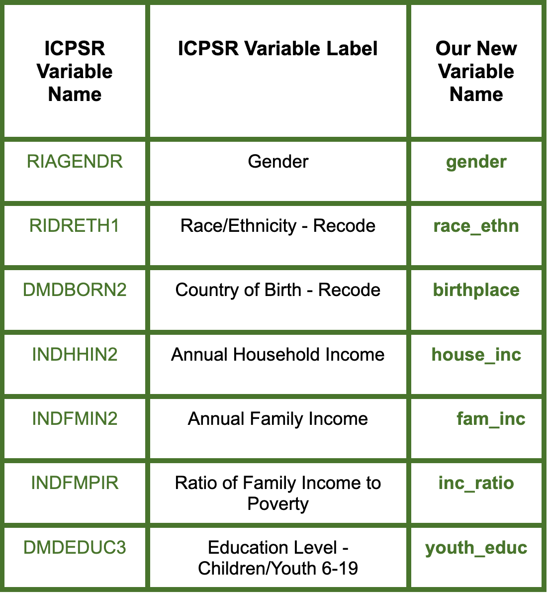
These are a few of the variables which we will be cleaning and processing throughout the rest of the guide. Let’s now rename them by using the rename command which has the following syntax

Listing all of the variables within the dataset allows us to see the updated variable names:

names(edited_NHANES)

Now that we have renamed five common variables, we can move on to making sure there aren’t duplicates within the dataset.

Checking for Duplicates

An important cleaning step when working with surveys meant to contain one observation per interviewee is to make sure that there aren’t duplicates.

To check whether or not there are duplicates under the SEQN variable which represents a respondent’s ID, we can run:

There are 9 duplicates under SEQN which should be removed. To remove the 9 duplicates, we can run:

We have now successfully deleted the 9 duplicates under respondent ID and can move on to removing outliers.

Removing Outliers

Identifying and removing outliers is an important step which can allow us to gain more accurate results from our analyses. Before we decide on an appropriate method for doing so, let’s learn about the distribution of our dataset.

Let’s narrow our focus specifically to the INCPERQ, or quarterly income variable, which we might expect to include outliers.

Using the quantile command in R and running the following:

We can observe that 25% of people made below $5,583, 50% below $10,949, 75% below $21,88, and 99% below 119,830 in the last quarter. Looking at the column which lists the largest values under the variable, we could get an idea of the values which should be considered outliers and subsequently dropped.

Let’s save the value assigned to the cutoff for the top 1% of quarterly income (INCPERQ), or those who indicated more than 119,830 in the last quarter as p99.

p99 <- quantile(unique_NHANES$INCPERQ, 0.99, na.rm = TRUE)

We can now see that our newly stored item has been populated under the ‘Values’ tab. Let’s move on to only saving values of INCPERQ which are less than p99.

unique_NHANES <- unique_NHANES[unique_NHANES$INCPERQ <= p99, ]

If we create another quantile breakdown using the quantile command, we can now see that the quantiles have been adjusted as a result of us dropping the highest values which were previously skewing the dataset.

Now that we’ve learned how to remove outliers, we can move on to examining our dataset’s proxy variables.

Assessing the Validity of Proxy Variables

In the context of the NHANES, there are variables which indicate whether the responses came directly from the respondent or someone else. These are MIAPROXY, SIAPROXY, and FIAPROXY. They represent whether a respondent used a proxy in the mobile examination center (MEC), sample person (SP), or family interview respectively. This means that instead of the individual, themselves, answering, they instead chose to elect a representative to answer in their place. This could significantly bias the dataset so we’d like to indicate where this was true.

Within your work with this survey, you might be interested in running certain analyses on just the responses from proxies and vice versa. In this case, we can make a new variable that codes ‘1’ for any of the three proxies and 0 otherwise.

Looking at the data allows you to view the new column that has been created to take the value of 1 for any of the three proxies being present.

Let’s now run some summary statistics to see how responses might differ between proxies and non-proxies. First, running tab allows us to see that proxies are used in around 36% of the responses in the dataset.

table(unique_NHANES$proxy)

Congrats on making it to the end of this ERC R How-To Guide!

Additional Sources:

How to: Merge Datasets in R